2.1: Alpha Diversity – Statistical Analysis of Metagenomic Data

Transforming data

Relative Abundance

Data is already normalized with sample sums ~ 100

This is used for Shannon, Simpson and Inverse Simpson as they are robust to sequencing depth if using relative abundances.

Normalize sequencing depth - rarefaction

Rarefaction (random subsampling without replacement).

In microbial ecology and amplicon sequencing (e.g., 16S rRNA gene sequencing) where samples often have vastly different numbers of reads. Rarefying aims to make all samples have the same total number of reads by randomly drawing a subset of reads from each sample without replacement. The chosen target depth is usually the smallest library size among all samples, so that no sample is asked to provide more reads than it originally had. This is only used for observed alpha diversity as rarefaction ensures each sample contributes the same number of reads.

source("inputData.R")


Attachement du package : 'dplyr'

Les objets suivants sont masqués depuis 'package:stats':

    filter, lag

Les objets suivants sont masqués depuis 'package:base':

    intersect, setdiff, setequal, union

library("vegan")

Le chargement a nécessité le package : permute

library("phyloseq")
# metagenomics_rel <- transform_sample_counts(metagenomics, function(x) x / sum(x))
# metagenomics_rel

# Test if rarefaction is needed for a phyloseq object (simple version)
test_rarefaction <- function(ps, cv_thresh = 0.05) {
  libs <- sample_sums(ps)
  cv <- sd(libs) / mean(libs)
  need <- cv > cv_thresh
  list(cv = cv, rarefy_recommended = need)
}

res <- test_rarefaction(metagenomics)
res$cv

[1] 0.0310323

res$rarefy_recommended # TRUE/FALSE

[1] FALSE

if(res$rarefy_recommended) {
  min_sample_size <- min(sample_sums(metagenomics))
  metagenomics_rare <- rarefy_even_depth(metagenomics, sample.size = min_sample_size)
  print("Rarefaction is recommended.")
} else {
  print("No rarefaction needed.")
}

[1] "No rarefaction needed."

Rarefaction

Calculate alpha diversity

# # alpha diversity for Shannon, Simpson, InvSimpson
# alpha_div <- estimate_richness(metagenomics, measures = c("Shannon", "Simpson", "InvSimpson"))
# p1 <- plot_richness(metagenomics, x = "disease", measures = c("Shannon", "Simpson", "InvSimpson"))
# p1
# ggsave("figures/Alpha/alpha_diversity_shannon_Simpson_invSimpson.pdf", p1)
# 
# alpha_obs <- estimate_richness(metagenomics, measures = c("Observed"))
# p2 <- plot_richness(metagenomics, measures = c("Observed"))
# p2
# ggsave("figures/Alpha/alpha_diversity_observed.pdf", p2)
# 
# alpha_df <- cbind(alpha_div, alpha_obs)
# alpha_df$SampleID <- rownames(alpha_div)
# alpha_df$Disease <- sample_data(metagenomics)$disease

# Manual calculation from relative abundances (works with fractions)
otu_rel <- as(otu_table(metagenomics), "matrix")
if (taxa_are_rows(metagenomics)) otu_rel <- t(otu_rel)

# Function to compute Shannon from relative abundances
shannon_from_rel <- function(x) {
  x <- x[x > 0]
  p <- x / sum(x)
  -sum(p * log(p))
}

# Function for Simpson (1 - sum(p^2))
simpson_from_rel <- function(x) {
  x <- x[x > 0]
  p <- x / sum(x)
  1 - sum(p^2)
}

# Function for Inverse Simpson (1 / sum(p^2))
invsimpson_from_rel <- function(x) {
  x <- x[x > 0]
  p <- x / sum(x)
  1 / sum(p^2)
}

# Apply to each sample
shannon <- apply(otu_rel, 1, shannon_from_rel)
simpson <- apply(otu_rel, 1, simpson_from_rel)
invsimpson <- apply(otu_rel, 1, invsimpson_from_rel)
observed <- apply(otu_rel, 1, function(row) sum(row > 0))

# Create data frame
alpha_df <- data.frame(
  SampleID = sample_names(metagenomics),
  Shannon = shannon,
  Simpson = simpson,
  InvSimpson = invsimpson,
  Observed = observed,
  Disease = sample_data(metagenomics)$disease
)

# Plot with ggplot2
library(ggplot2)
library(tidyr)

# Reshape for faceting
alpha_long <- pivot_longer(alpha_df, cols = c(Shannon, Simpson, InvSimpson, Observed), names_to = "Metric", values_to = "Value")

p_combined <- ggplot(alpha_long, aes(x = Disease, y = Value, fill = Disease)) +
  geom_boxplot() +
  facet_wrap(~Metric, scales = "free_y") +
  theme_bw() +
  labs(title = "Alpha diversity from relative abundances")

p_combined

# ggsave("figures/Alpha/alpha_diversity_all.pdf", p_combined, width = 10, height = 6)

\(R\) = total number of taxa in the community

\(p_i\) = relative abundance of taxon \(i\)

\(I\) = = indicator function (1 if taxon is present, 0 otherwise)

Observed richness: \(S = \sum_{i=1}^{R} I(p_i > 0)\)

Shannon diversity: \(H' = -\sum_{i=1}^{R} p_i \ln(p_i)\)

Simpson index: \(D = \sum_{i=1}^{R} p_i^2\)

Inverse Simpson: \(1/D = 1 / \sum_{i=1}^{R} p_i^2\)

Normality Testing

# Check Normality (Shapiro-Wilk) to decide test 
shapiro.test(alpha_df$Shannon)


    Shapiro-Wilk normality test

data:  alpha_df$Shannon
W = 0.94912, p-value = 7.577e-12

shapiro.test(alpha_df$Simpson)


    Shapiro-Wilk normality test

data:  alpha_df$Simpson
W = 0.75802, p-value < 2.2e-16

shapiro.test(alpha_df$InvSimpson)


    Shapiro-Wilk normality test

data:  alpha_df$InvSimpson
W = 0.97731, p-value = 7.625e-07

shapiro.test(alpha_df$Observed)


    Shapiro-Wilk normality test

data:  alpha_df$Observed
W = 0.98674, p-value = 0.0002161

If p-value > alpha 0.5, data is normal, use ANOVA. All test rejects the null hypothesis, so we use non-parametric test (Kruskal-Wallis).

Shapiro–Wilk tests assess whether diversity metrics follow a normal distribution. In microbiome datasets, these metrics are typically non-normal due to compositionality and sparsity. Therefore, results are used as a diagnostic tool rather than a strict decision criterion.

kruskal.test(Shannon ~ Disease, data = alpha_df)


    Kruskal-Wallis rank sum test

data:  Shannon by Disease
Kruskal-Wallis chi-squared = 65.355, df = 3, p-value = 4.212e-14

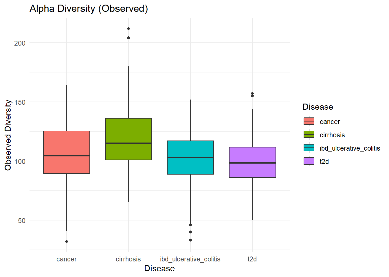
kruskal.test(Observed ~ Disease, data = alpha_df)


    Kruskal-Wallis rank sum test

data:  Observed by Disease
Kruskal-Wallis chi-squared = 48.651, df = 3, p-value = 1.548e-10

kruskal.test(Simpson ~ Disease, data = alpha_df)


    Kruskal-Wallis rank sum test

data:  Simpson by Disease
Kruskal-Wallis chi-squared = 57.58, df = 3, p-value = 1.932e-12

kruskal.test(InvSimpson ~ Disease, data = alpha_df)


    Kruskal-Wallis rank sum test

data:  InvSimpson by Disease
Kruskal-Wallis chi-squared = 57.58, df = 3, p-value = 1.932e-12

The Kruskal–Wallis test evaluates whether median diversity differs across disease groups without assuming normality. A significant result indicates that at least one group differs, but does not specify which groups differ.

Alpha Diversity Visualization

p3 <- ggplot(alpha_df, aes(x = Disease, y = Shannon, fill = Disease)) +
  geom_boxplot() +
  theme_minimal() +
  ylab("Shannon Diversity") +
  xlab("Disease") +
  ggtitle("Alpha Diversity (Shannon)")
# ggsave("figures/Alpha/alpha_boxplot_shannon.pdf", p3)
p3

p4 <- ggplot(alpha_df, aes(x = Disease, y = Simpson, fill = Disease)) +
  geom_boxplot() +
  theme_minimal() +
  ylab("Simpson Diversity") +
  xlab("Disease") +
  ggtitle("Alpha Diversity (Simpson)")
# ggsave("figures/Alpha/alpha_boxplot_Simpson.pdf", p4)
p4

p5 <- ggplot(alpha_df, aes(x = Disease, y = InvSimpson, fill = Disease)) +
  geom_boxplot() +
  theme_minimal() +
  ylab("InvSimpson Diversity") +
  xlab("Disease") +
  ggtitle("Alpha Diversity (InvSimpson)")
# ggsave("figures/Alpha/alpha_boxplot_InvSimpson.pdf", p5)
p5

p6 <- ggplot(alpha_df, aes(x = Disease, y = Observed, fill = Disease)) +
  geom_boxplot() +
  theme_minimal() +
  ylab("Observed Diversity") +
  xlab("Disease") +
  ggtitle("Alpha Diversity (Observed)")
# ggsave("figures/Alpha/alpha_boxplot_Observed.pdf", p6)
p6

Alpha Diversity Plot Interpretation

Shannon

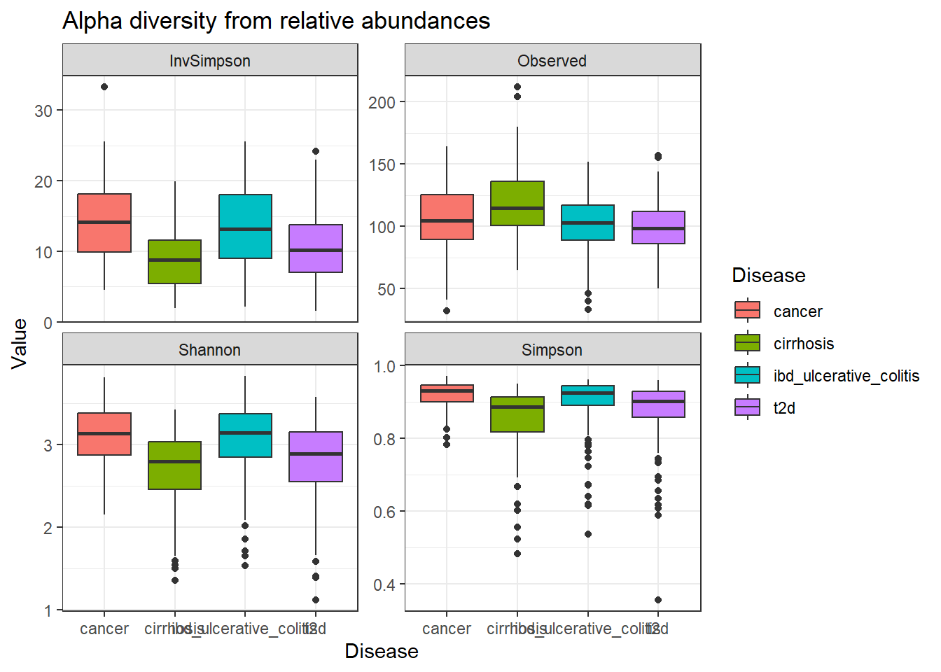
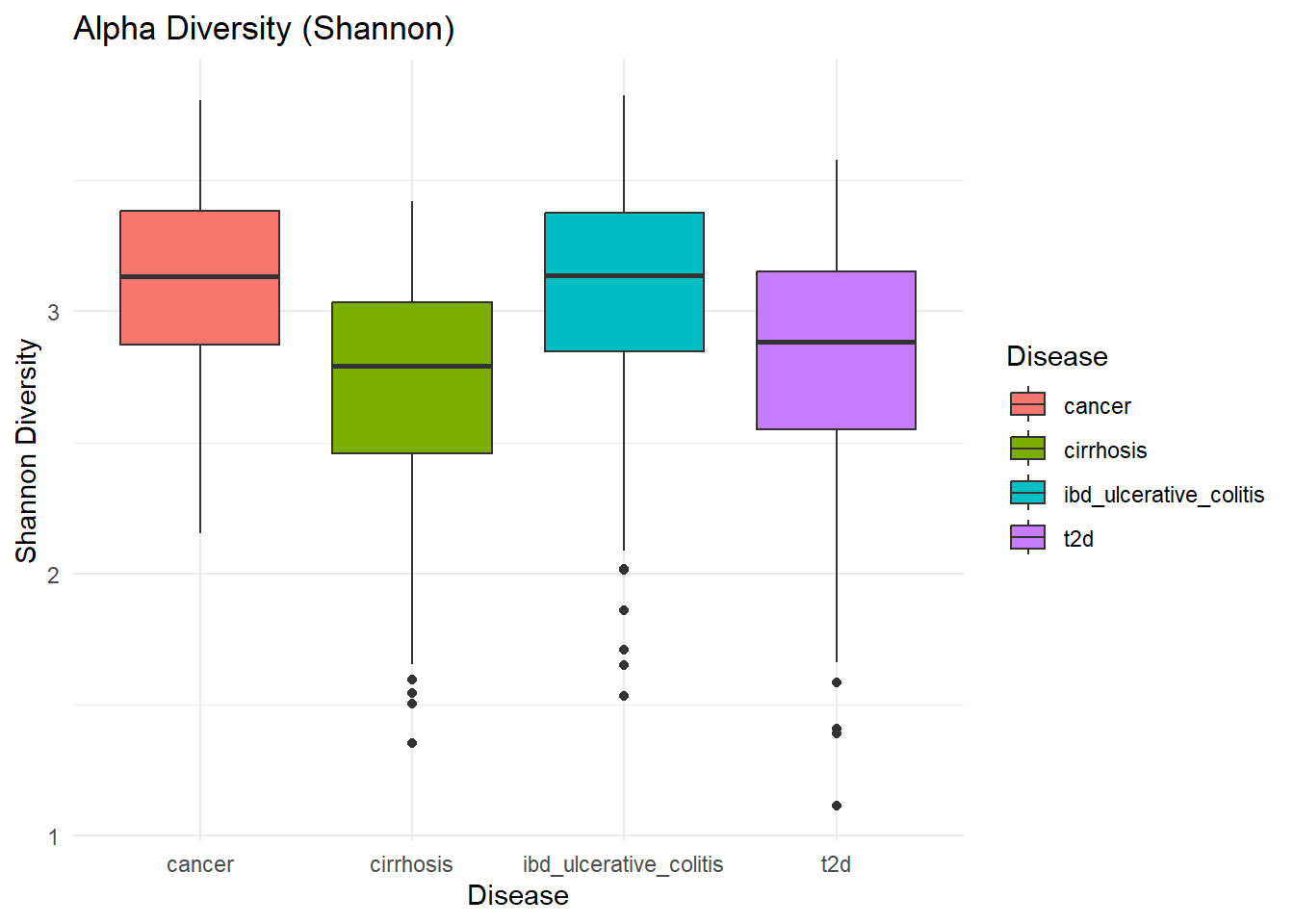
A popular way to measure the diversity of species in a community. It takes into account both species richness and species evenness. It is calculated based on the logarithm of the relative abundances of species in a community. Higher values of Shannon Diversity indicate higher species richness and evenness. In general, values of 3.50 and above for Shannon-Wiener index indicates high diversity while values below 2.0 indicate low diversity (Baliton et al., 2020).

Simpson

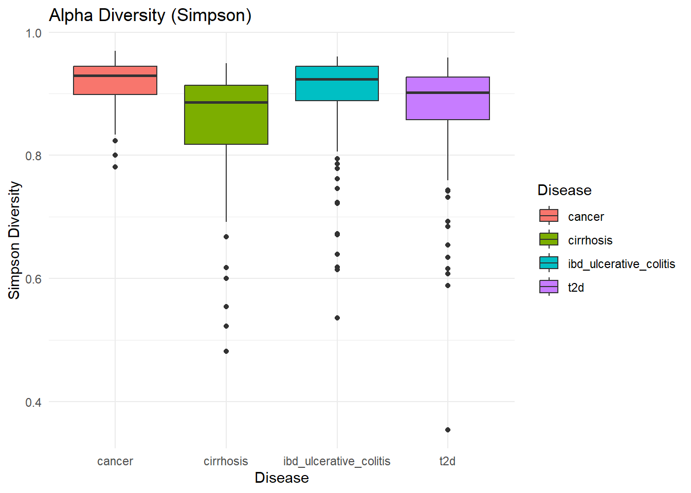
The Simpson Index is a measure of diversity that quantifies the probability that two randomly selected individuals from a community belong to the same species. It ranges from 0 to 1, with higher values indicating lower diversity. It is often used to assess the dominance of a few abundant species in a community. The value of D ranges between 0 and 1. The value of Simpson’s D ranges from 0 to 1, with 0 representing infinite diversity and 1 representing no diversity, so the larger the value of D, the lower the diversity.

Inverse Simpson

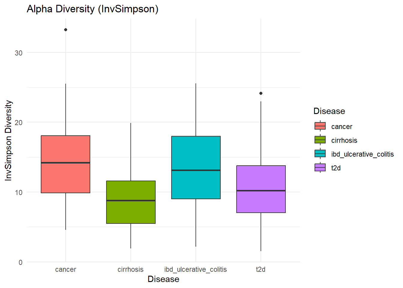
It is the reciprocal of the Simpson Index and is often used to emphasize the importance of rare species in a community. Higher values indicate greater diversity. It is positively correlated with the Shannon index.

Observed

Counts the actual number of unique features (OTUs) present.

Post-Hoc

Since Kruskal-Wallis tells you there’s a difference somewhere among the groups, we may want to do post-hoc pairwise comparisons to see which groups differ. For non-parametric tests, we can use:

library(FSA)

## FSA v0.10.1. See citation('FSA') if used in publication.
## Run fishR() for related website and fishR('IFAR') for related book.

# Pairwise Wilcoxon test with p-value adjustment
pairwise.wilcox.test(alpha_df$Observed, alpha_df$Disease, p.adjust.method = "BH")


    Pairwise comparisons using Wilcoxon rank sum test with continuity correction 

data:  alpha_df$Observed and alpha_df$Disease 

                       cancer cirrhosis ibd_ulcerative_colitis
cirrhosis              0.019  -         -                     
ibd_ulcerative_colitis 0.279  3.9e-07   -                     
t2d                    0.074  7.9e-11   0.158                 

P value adjustment method: BH

pairwise.wilcox.test(alpha_df$Simpson, alpha_df$Disease, p.adjust.method = "BH")


    Pairwise comparisons using Wilcoxon rank sum test with continuity correction 

data:  alpha_df$Simpson and alpha_df$Disease 

                       cancer  cirrhosis ibd_ulcerative_colitis
cirrhosis              1.3e-06 -         -                     
ibd_ulcerative_colitis 0.80457 4.6e-10   -                     
t2d                    0.00037 0.01071   2.8e-06               

P value adjustment method: BH

pairwise.wilcox.test(alpha_df$InvSimpson, alpha_df$Disease, p.adjust.method = "BH")


    Pairwise comparisons using Wilcoxon rank sum test with continuity correction 

data:  alpha_df$InvSimpson and alpha_df$Disease 

                       cancer  cirrhosis ibd_ulcerative_colitis
cirrhosis              1.3e-06 -         -                     
ibd_ulcerative_colitis 0.80457 4.6e-10   -                     
t2d                    0.00037 0.01071   2.8e-06               

P value adjustment method: BH

pairwise.wilcox.test(alpha_df$Shannon, alpha_df$Disease, p.adjust.method = "BH")


    Pairwise comparisons using Wilcoxon rank sum test with continuity correction 

data:  alpha_df$Shannon and alpha_df$Disease 

                       cancer  cirrhosis ibd_ulcerative_colitis
cirrhosis              9.1e-08 -         -                     
ibd_ulcerative_colitis 0.689   1.1e-10   -                     
t2d                    2.6e-05 0.046     1.6e-07               

P value adjustment method: BH

# p.adjust.method = "BH" → controls for multiple comparisons (Benjamini-Hochberg FDR)

Wilcox test identifies specific group differences following a significant Kruskal–Wallis result. The Benjamini–Hochberg correction controls the false discovery rate due to multiple pairwise comparisons.

Summary

Alpha diversity analysis evaluates whether microbial community structure differs between disease groups in terms of richness and evenness. If significant differences are observed across metrics, this suggests that disease status is associated with broad ecological shifts in the microbiome, such as loss of diversity, increased dominance, or reduced richness.

Consistency across multiple indices strengthens biological inference, while divergence between metrics may indicate changes in community structure rather than simple loss or gain of taxa.

Alpha diversity was assessed using Shannon, Simpson (1 − D), Inverse Simpson, and Observed richness indices computed from relative abundance data. Differences between disease groups were tested using Kruskal–Wallis tests followed by Wilcox post-hoc tests with Benjamini–Hochberg correction. Normality assumptions were evaluated using Shapiro–Wilk tests for exploratory purposes only.